What are Neural Oscillations?

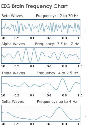
Neural oscillations are repetitive, rhythmic synchronized frequency patterns in the central nervous system. They occur during activation of large clusters of neurons, though they can occur with a single neuron as well. Although the raw data obtained from electroencephalograms are formatted as a function of time, neural oscillations are visualized in terms of frequency and measured in units of Hertz (Hz); one cycle per second. As such the neural clusters generate neural oscillations that can be characterized by the frequency range in which they occur:

• Alpha waves (7.5-12.5 Hz) are commonly associated with cognitive functions such as attention and awareness. Alpha waves are also linked with learning processes and are the most common freqency analyzed in mood / meditation apps.
• Beta waves (13-30 Hz): These waves are commonly associated with concentration / attention.
• Delta waves (1-4 Hz): These high amplitude waves are linked with slow-wave sleep (SWS).
• Gamma waves (30-70 Hz): Gamma wavs are fast waves associated with attention, concsiousness and perception.
• Mu waves (7.2 - 12.5, primarily 9 - 11): These waves are located over the motor cortex and are primarily associated with a state of physical rest. They are desynchronixed (a.k.a. suppressed) during a motor action.
• Theta waves (4-8 Hz): Two types of theta oscillations have been described based on the location of their occurence. The hippocampal theta rhythm is a strong oscillation that can be observed in the hippocampus, while the cortical theta rhythms are low-frequency components of scalp EEG. There is no clear understanding of the function of theta waves, however a combination of several theories supports that hippocampal theta waves are linked to navigation and memory. Cortical theta waves are observed more frequently in young children and appears during meditative, drowsy,hypnotic, and non-deep sleeping states.

Why do we produce neural oscillations?

We do not fully understand why our brain produces neural oscillations. Some researchers theorize that neural oscillations are nothing more than byproducts of brain activity, indicators of expected brain pattern in response to events of stimulus. For example, motion produces predictable occurrences of alpha waves (in the mu frequency) in the motor cortex, and sleep cycles are characterized by the alternating flux of different neural waves. Other researchers have theorized that certain oscillations, like those that occur in the delta range, are critical to unlocking the mystery of our consciousness.

So why do neural oscillations matter?

Neural oscillations are useful in variety of ways. From a diagnostic and imaging perspective, they can be used as indicators of specific neurological phenomena such as:

• Sleep and the state of consciousness
• Motor control
• Perception and information processing
• Pattern generation
• Memory
• Abnormal neural function, such as epilepsy, and Parkinsons.

Practical applications for extracting neural oscillations using your own BCI could be looking at the presence of mu waves during motion, or to check if there is a presence of alpha and beta waves during meditation. You may even want to look at all the different waves that occur when you are performing a specific task.

How do we extract neural oscillations as a feature of our EEG data?

As previously mentioned data obtained by EEF are captured as a function of time, but neural oscillations are described in units of frequency. In order to transform data we must employ a Fourier transform.

The Fourier transform is a highly regarded formula which is the mainstay formula for signal processing and signal decomposition. If you would like to learn more about the Fourier transform and FFT, I recommend this video. It’s a little long but it’s worth the watch!

The best way to extract neural oscillations is to perform a Fourier transform on your preprocessed data and then plot the resulting frequency patterns in the category of brain waves your interested in seeing. You can further preprocess your data to exclude certain channels, or target specific frequency ranges to observe features of the neural oscillation. See NeuroTechX.edu “Preprocessing” for a detailed look at the preprocessing steps that can be applied to your data.

Before extracting neural oscillations there are several steps that must be undertaken to prepare you data:

• Importing data, reading data, and formatting data
• Preprocessing
• Epoching
• Assemble a classifier (plotting a topomap)
• and finally, plotting the relevant figure

Importing, reading, and formatting data

In the below example I have used a dataset created by experimental runs by (research reference) so when data is fetched it will have already underwent some preprocessing which will not be covered in either examples. However in both cases data will be fetched using the below commands:

subject = 1
runs = [3]
tmin = -0.1
tmax = 0.3
raw_fnames = eegbci.load_data(subject,runs)
raw_files = [read_raw_edf(f, preload=True) for f in raw_fnames]
raw = concatenate_raws(raw_files)
raw.ch_names.index('STI 014')

The above code can be broken down into two components. Line 1 - 4 set parameters to define which parts of the dataset are to be analyzed, while line 5-8 pulls data and connects what it does (What do these lines actually do?)

Line 2 is relevant in this example, as there are 14 experimental runs to choose from that were performed in this study and each was tested under different conditions. In this experiment run 3 measured the EEG signal obtained during movement of the left and right hands, both separately and simultaneously.

Preprocessing

Preprocessing is a critical step when analyzing EEG data. EEG data contains a lot of noise, and data that are not relevant to what you’re attempting to visualize. Preprocessing is a deep topic and there are many ways you can go about cleaning up EEG data. Check out our post on preproccessing [here]{http://learn.neurotechedu.com/preprocessing/}. When plotting power spectral density (psd), only epoching is necessary as we want to see the psd across the entire available frequency range. However for topomap plotting you will need to preprocess your data with a band pass filter to isolate the specific frequency range you want to visualize. The example below also strips the channel names of their default “.” keys to avoid errors when reading your channel names.

Epoching data

Epoching is dividing data into segments of data based on a timeframe of interest. The interest is generall determined by an event whether an evoked event or an induced event. (do we have a segment of information that explores epoching more in depth?). To epoch your data you can follow the steps below:

events = mne.find_events(raw, stim_channel='STI 014', verbose=True)
picks = pick_types)raw.info, meg=Fale, eeg=True, stim=False, eog=False, exclude='bas')
baseline = 0, None

The above defines the events you want to look for, as well as the type of signal your program should expect to analyze (meg vs. eeg vs. eog). I selected the eeg=True as data we will be looking at were obtained using an EEG headset. Below we continue the necessary inputs for epoching:

epochs = Epochs(raw, events, event_id, tmin, tmax, proj=True, picks=picks, baseline-baselin, preload=True)
epochs_train=epochs.copy().crop(tmin=-0.2,tmax=0.5)
labels=epochs.events[:,-1]-

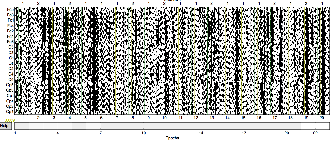
The above code defines the epochs which will be further manipulated. Try the function plot.epochs() to see how your data have transformed! (Hint: It might look something like the image below!)

The following steps will diverge depending on the methods of visualization you want to apply. Below I will highlight how to use psd to visualize dominant frequencies as well as topomaps to highlight specific frequencies in localized areas.

Using PSD to categorize oscillatory occurrence based on power spectral content

Power spectral density measure the power of a signal in microvolts. The function epochs[events].plot_psd() can be used to plot specific epoched events as a function of power spectral density over a specific frequency range. Below is an example of a script you can run to achieve this. Note that the dataset imported from eegbci is already preprocessed and transformed using the Fourier function, so the steps you should see below are:

• Importing, read, and format your data
• Epoch data
• Plot data with the epochs[events].plot_psd()

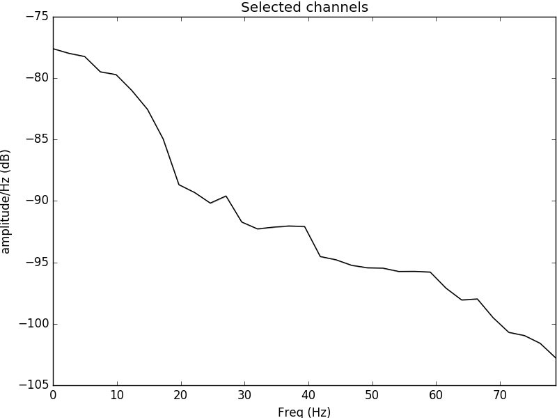
Figure 1: Power spectral density plotted for the electrode C3 located in the left side of the motor cortex. It is evident that the psd content is most evident in the alpha range and theta range, evident of neural oscillations occurring during movement of the right hand.

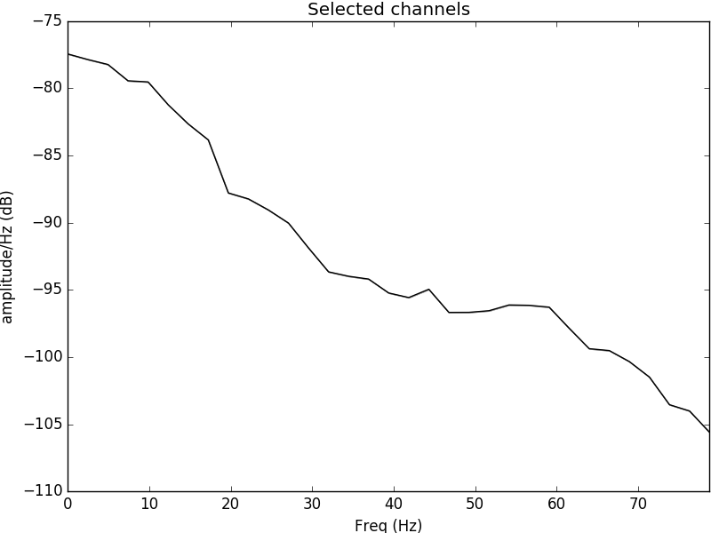
Figure 2: Power spectral density plotted for the electrode C4 located in the left side of the motor cortex. It is evident that the psd content is most evident in the alpha range and theta range, evident of neural oscillations occurring during movement of the left hand.

Using a topomap to visualize local oscillations

Quick highlights of topopmap

• A classifier will be applied to visualize the presence of neural oscillations using a binary discrimination to highlight whether you have the presence of waves at certain frequencies or not. While there is a bit of variability on visualizing the strength of your signal, this is really simply a “there” or “not there” method of looking at neurons firing over specific electrodes. Understanding which electrodes correspond to which regions of the brain will help you to understand where the majority of activity is occurring in the brain.

Plotting PSD to visualize frequency is limited to specific channels and may require excess work to view the local presence of waves. By contrast, topomap offers specific feedback on the local presence of waves. The classifier assembled in the below example uses a binary range characterized by the red positive values and the blue negative values. The total range is from -0.1 to 1.0 and refers to the electric potential with 1.0 indicating the presence of a measurable signal.

There are several more steps involved with topomap visualization. The first occurs in the preprocessing step as you must apply a band pass filter (raw.filter(fmin,fmax)) to isolate the frequency range that interests you. Refer to the above section where I break down each wave into their respective frequency range. The below example will be using a band pass filter for alpha and beta waves since the eegbci dataset runs are based on on motor cortex activity.

Five arbitrary time points were chosen in the below example to highlight the shift in wave presence over time. Since the run involves squeezing the right and left hands, we should expect an increase in the alpha wave presence (specifically the mu frequency) and a reciprocal decrease in beta wave frequency in the area corresponding to either right or left hand (opposite sides of the brain from the hand involved). Timepoints 4 and 5 illustrate this difference:

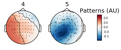
Figure 3: Topomap of alpha waves (7.5-12.5 Hz) during movement.

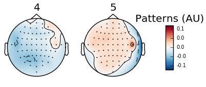
Figure 4: Topomap of beta waves (13-30 Hz) during movement.