Neurotechnology
Machine Learning for BCI
Machine Learning for Brain Computer Interfaces
Table of Contents
Introduction
Welcome to the NeurotechEDU Machine Learning BCI tutorial! We will introduce the fundamentals of classifying neurophysiological sensor data. This tutorial can be used in tandem with knowledge gained from the earlier tutorials to enhance the results we obtain here. We will introduce an example problem to solve, provide basic theory on why we will solve our problem with Neural Networks, and work out the solution within a Google Collab document. While this will be a basic tutorial focusing on one specific example, advanced topics will be occasionally discussed and further material can be found in other NeurotechEDU tutorials.
Let’s get started.

Source: https://medium.com/svilenk/bciguide-246a9ca76fcd –>
Quick Link
If you would like to skip ahead to the implementation, use this link:
Introducing a Problem
The difference between problems in a textbook and problems in the real world comes down to the issue of complexity. Real problems are rarely simple (and when they are, they’re not called problems anymore).
In order to solve these real problems, scientists will often create a simplified model system to build theories about the complex model. However, inferring patterns and theories is error-prone, difficult, and very, very slow.
To hang an example onto this difficult topic, it would be easy to look at a global economy. Untold amounts of variables exist that drive the stock tickers we see on the news every day. Variables range from complex trading strategies of the world-leading investment firms down to the level of risk aversion of a single trader.
Our brains are not equipped to logically understand that level of complexity, which is why we employ machine-run algorithms to give a thorough estimation to the solution of these complex problems with relative speed and precision.
Interfaces to Brains
Ironically, human brains themselves are another such complex system. Signals gathered from sensors reading voltage levels are as indirect to actual brain interfacing as we can get. However, it’s currently the best we can do without invasive methods that require electrodes that go under the scalp.
To add on to that issue, everyone’s brain structure is different. Any single solution we find to our interfacing problem will not work for everyone. Interfaces we may develop need to be tailored to the individual, and the “problem” we’re solving by interfacing with their brain will change significantly. There is no one-size-fits-all solution and it is unlikely there ever will be, even with the extremely accurate sensors.
The Problem
For this tutorial, we will introduce a simplified problem and use a simple Neural Network to solve. To help us with this journey, we’ll be using a dataset provided on the MNE python library. This dataset provided a number of EEG samples that contain 226 data points per sample. Where each sample represents a single trial described in the problem. Below is a graph of two such plotted samples, with the channel displayed on the top right of the graph.
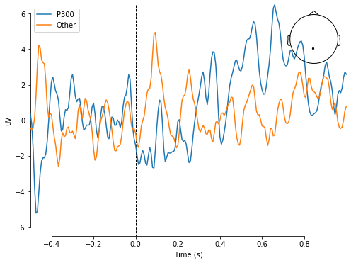
Image generated from the Google Collab Tutorial.
Problem Statement
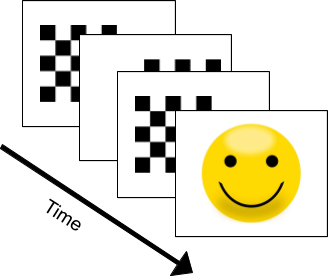
- Suppose we have a subject seated and viewing a screen with a set of images being displayed. In this experiment, checkerboard patterns were presented to the subject into the left and right visual field, interspersed by tones to the left or right ear. The interval between the stimuli was 750 ms. Occasionally a smiley face was presented at the center of the visual field. The subject was asked to press a key with the right index finger as soon as possible after the appearance of the face.
- Using only the EEG data feed provided, detect when the subject is shown the Smiley Face image, before they press the key.
The purpose of this experiment is to monitor the “surprise” or “anticipation” response. This response is commonly indicated by a well-researched EEG response called P300 component. If we create a system to detect this component within the EEG data feed, we will find the solution to our problem statement.
What is the P300?
We introduced the P3 component previously in a previous tutorial: http://learn.neurotechedu.com/erp/#the-p3-family-of-erps. To summarize, the P3 is a spike, or a positive deflection, that appears on our brainwaves around 300 ms after we observed a rare or targeted stimulus. For example, it will appear on your EEG data feed if someone draws a card that you were expecting from a deck.
A direct application of the P300 on BCI applications is the P300 speller. This application allows a person to type by selecting letters from an alphabet displayed on a screen just by focusing on the letter they are intending to type. An example of the P300 speller can be seen here: https://www.youtube.com/watch?v=XIr2cRKFolY (Starting in minute 2:00)
Using the P300 to detect events is a straightforward technique, but as we’ll discover later detecting one without using an averaged value can actually be very difficult.
Introduce Machine Learning
Now that you’ve been introduced to the concept of Difficult Problems, we will also introduce one method that was created to make a dent in solving them. Machines are very good at following rules to identify patterns in these complex scenarios, and scientists have developed techniques to identify patterns and discern features that would be otherwise undetectable to a human being.
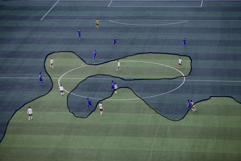
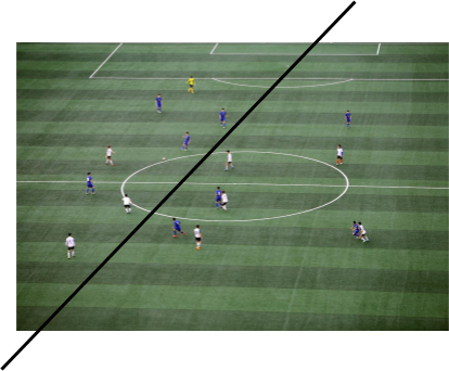
Let us imagine we are watching a football game and we paused the television on an aerial shot. What if we wanted to be able to predict what team is a player in just from where they are standing on the field. How could we do this? The easiest way is to draw a curve between the two teams. This is illustrated by the figure below.
Now, imagine that the teams are actually playing Quidditch and the player positions were now defined by three-dimensional coordinates instead of just two. In this new case, we would now require a 3D curve to separate the teams.
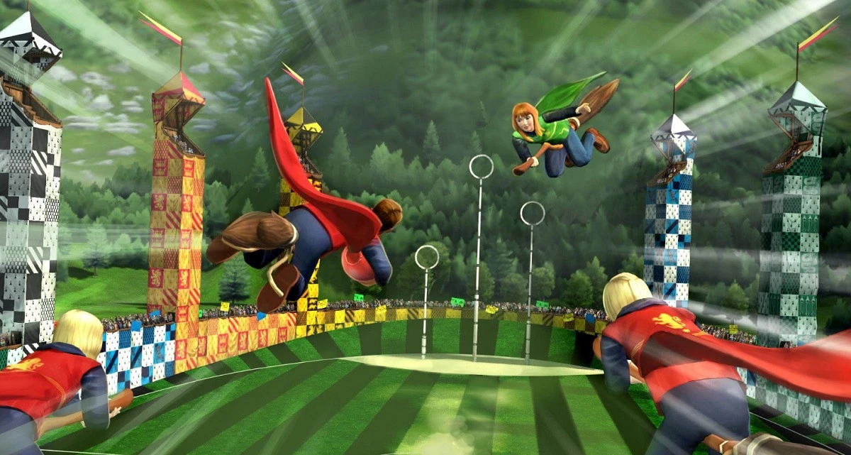
If we also consider the players’ positions relative to the time they occupy them, we would then have a four-dimensional problem which would require a 4-dimensional curve. This is much more difficult, maybe even impossible, to visualize.
Now let’s bring it back to our P300 problem. We have 226 data points, each of them would be considered a different dimension to the data. Why is this not a two dimensional problem, like the one we see in the figure below?
You can see in this figure the two types of brain waves overlap. However if we want to represent these brain waves in the same way we represent the football players, then we would have to place the wave as a single point inside of a 226 dimensional space. Then once we have a set of brain waves placed in that 226 dimensional space, we can create a 226 dimensional curve that separates them, just like the previous problem.
Not only is that space impossible to capture in a single picture, the complexity of the solution increases exponentially for every added dimension! In order to solve problems of this magnitude, we’ll need the assistance from a collection of mathematical tools that excels in solving high dimensional problems. When we look at the brain waves, we see data points over time. However, when this is processed by a machine learning algorithm, the whole brainwave is represented as a single point. Each brain wave will be plotted this way, and we will try to find a function in that dimensionality that will separate the P300 from the regular brainwaves.
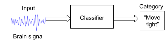
Machines can work in any number of dimensions which can be hard for humans to visualize. And as such, they have the ability to make predictions in a way that would be far too difficult for even an army of mathematicians to accomplish. In the context of Brain Computer Interfaces, machine learning is mostly used to develop classifiers. For example, a classifier could receive brain signal as an input, and put labels on it, like “Move right”.
Many different machine learning algorithms exist, but let’s focus on the few common tried-and-true algorithms that can help us solve our problem. The following are the most common algorithms found across BCI applications.
Support Vector Machine (SVM)
In general terms, SVM algorithms, just like other machine learning techniques, aim to define a curve capable of differentiating two distinct classes of data. In a higher dimensional space, this curve is called a hyperplane. In order to find the correct hyperplane, the algorithm goes through an optimization process where the number of misclassified instances (players, in the above example) are minimized. This process is what we call “training the algorithm” and we’ll go over how to do it later in this tutorial.
Something to keep in mind is that the simplest solution to classify 2 different types of items, like the two teams on our example, is to draw a line between them, for example:
In the problem we’re solving in this tutorial, we want to detect if a user is seeing something surprising based on their EEG signals. In order to do that, we will need data samples of brainwaves containing the P300 component and not containing the P300 component (which will be our two classes) to train the algorithm. The data we will feed to the SVM will be the values obtained for each of the channels on our EEG assembly.
The SVM optimization process will try to work towards three different goals with descending importance:
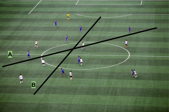
Rule 1: Minimization of misclassified instances. This is the main objective of the hyperplane. However, there will be cases when it is not possible to find a hyperplane that separates all the classes correctly, and based on that we can define the accuracy of our algorithm. In the figure below, line A represents a better SVM than line B.
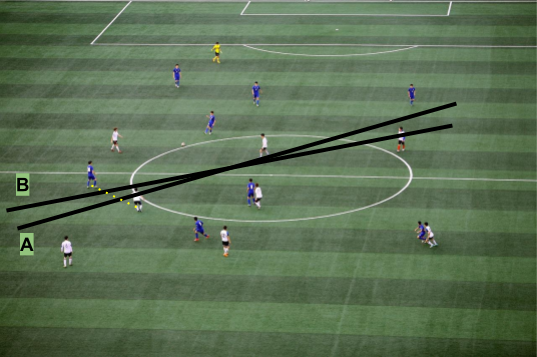
Rule 2: The hyperplane must maximize the distance to the nearest point of either of class labels. In other words, if the hyperplane could be located further apart from an example (without affecting rule 1), it should do it. In the figure below, line A should be considered over line B.
Rule 3: When one line is not capable of separating one class from the other (for example when the points of one class are surrounding the other class points), SVM’s can also use something called the ‘kernel trick’. In this case the SVM algorithm uses some mathematical transformations in order to place the classes of data on different levels, which will help to find a hyperplane that meets the required condition. There are several kernels available, however the most commonly used is the Radial Basis Function (BRF). The example shown at the beginning of the SVM section is an example of a problem that cannot be solved with a line, but using a kernel trick, we might be able to find the real boundary between the two teams.
Note: The hyperplane that the SVM is trying to find is known as the maximum-margin hyperplane.
Some important aspects to consider when implementing SVM algorithms are:
- Features should always be numeric.
- When the features are normalized and standardized, the algorithm’s performance could increase considerably.
Neural Networks
There’s nothing more suitable to learn how to solve a problem than a brain. Neurons fire in sequence and further cause a chain reaction of other neurons firing which in turn creates a cascade effect and results in all the things that a brain can accomplish. Neural networks are modelled after this behavior and attempt to replicate the ability of a human brain to learn how to solve a problem.
Below is a side-by-side of the first proper depiction of neurons and the neural network we create in this tutorial. It’s easy to see the resemblance of their structures.
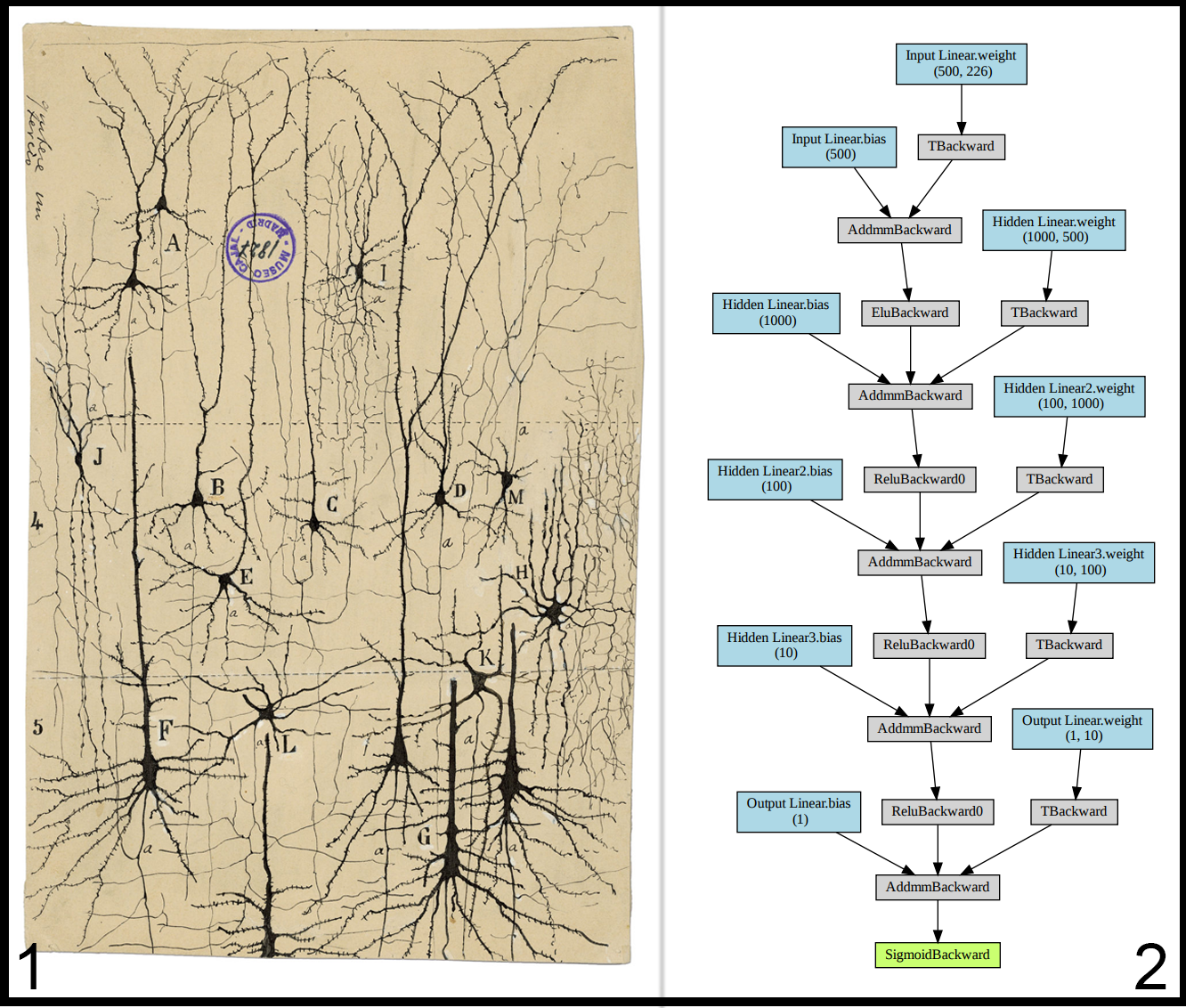
Each neuron in a brain has inputs (dendrites) connected to the outputs (axons) of other neurons. The neuron is constantly receiving signals from other neurons up the line, and if these signals surpass a firing threshold, then the neuron propagates that signal along its axon to other neurons further down. Not all neurons are connected in the same way, where some neurons might have stronger connections than others. This is defined as the weight of the connection. Neural networks work identically. Each neuron in a neural network is associated with a weight and something called an “activation algorithm” (see below), which ultimately decides what scale of output is created when a certain accumulated amount of input is received.
Much like the SVM, the Neural Network is creating a multi-dimensional solution space that curves and warps in an attempt to create a “best fit” solution to classify the data. However, neural networks require training and come up with the solution algorithm on their own. SVMs begin with an algorithm already decided. This means that Neural Networks require more setup time, but generally are more flexible and effective.
In this tutorial, we don’t have a perfect equation to represent p300 components. Additionally p300 components may manifest differently depending on what subject the EEG data is taken from, as well as a possibility of nonlinear noise. We need an algorithm that is able to adapt to those possibilities as well as other more subtle problems we may not not have encountered yet. We will show you how to train and deploy a neural network capable of identifying p300 components, and in turn solve our initial problem of identifying when a subject is surprised by some image.
Neural networks are very small in scale compared to the sheer size of the structures found within the brain. Only a few neurons are used to encode the input and the output.
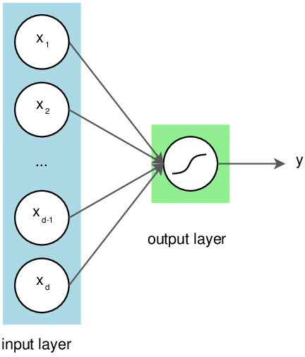
Above: This kind of neural network can only solve linear problems
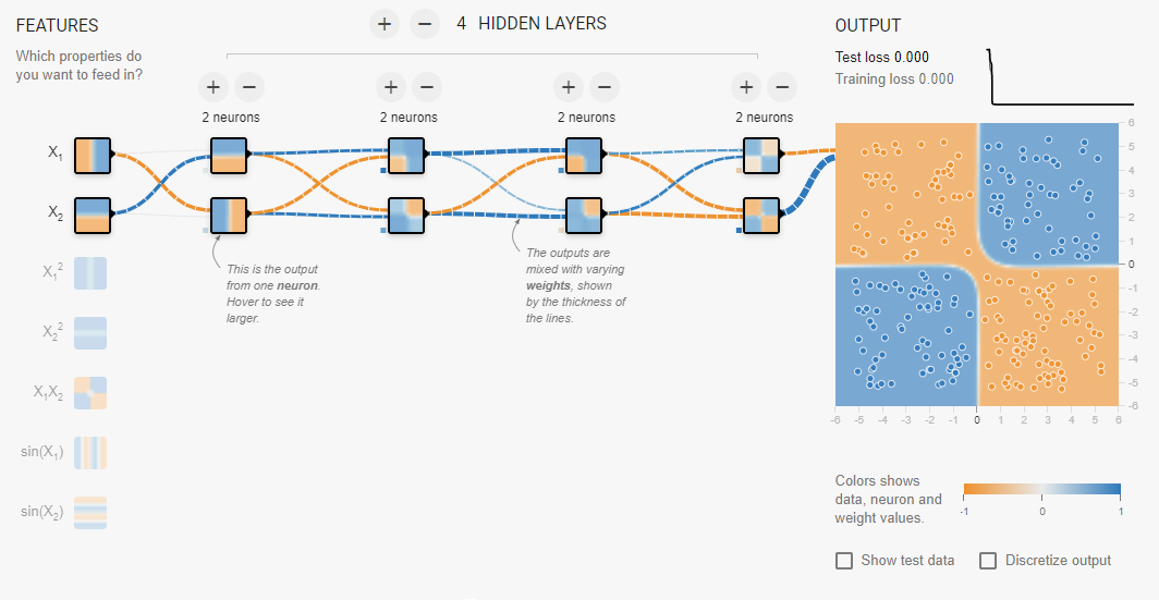
But for problems where the categories might mix, a non-linear approach is necessary. This is the essence of the “XOR Problem” that plagued early machine learning theorists. The solution to this was found to be fairly simple. Just add more layers to the network!
Implementing a Network
Ok enough talk, let’s do this. All the steps in this tutorial can be followed through our Google Collab document and tinkerers can either copy the document to their Google Drive or download the python file to run it locally.
From there, you can click on File and “Save a copy to Drive…” or “Download .py” to your preference. The tutorial is also shown here. Structures and methods within the tutorial can be modified to suit the curious mind.
This tutorial will go through the steps of creating and training a neural network on EEG data. Installation instructions are provided if you would like to follow along locally, but all steps are shown with their respective outputs in this Collab document.
(Step 1) Set Up the Environment
Before we begin, please ensure that you have a local Python version of at least Python 3.5 or greater. If you do not have a compatible Python version yet, please see the Python Beginners Guide for installation instructions
The prerequisite packages to this tutorial are:
- MNE: EEG Data Package
- NumPy: Scientific Computing (SciPy Download Page)
- SciPy: Scientific Computing
- MatPlotLib: Plotting Library
- Scikit-Learn: Machine Learning Library
- PyTorch: Machine Learning Library
Below is a pip script that installs these libraries on Google Collab. If any do not work, please see their respective installation pages.
# Run these from the console if following along locally
!pip install mne
!pip install sklearn
!pip install matplotlib
!pip install torch
!pip install torchvision
!pip install tensorboardX
For the purposes of this tutorial, we will be turning off warnings.
# You'll want to comment this out if you plan on modifying this code, to get valuable feedback
import warnings
warnings.filterwarnings('ignore')
Import all of our required modules. This includes various submodules that we’ll need including the RobustScaler object from scikit.
from collections import OrderedDict
from pylab import rcParams
import torch
import torch.nn as nn
import torchvision.transforms
import matplotlib.pyplot as plt
import numpy as np
import mne
from sklearn.preprocessing import RobustScaler
Set the randomizer seed for some consistency
torch.manual_seed(100)
(Step 2) Initialize Parameters
Initialize our project with a few constant parameters.
- eeg_sample_count: Number of samples we’re training our network with
- learning_rate: How fast the network tends to change its weights
- eeg_sample_length: Number of datapoints per sample
- number_of_classes: Number of output classes (1 output variable with 1.0 = 100%, 0.0 = 0% certainty that this sample has a p300)
- hidden1: Number of neurons in the first hidden layer
- hidden2: Number of neurons in the second hidden layer
- hidden3: Number of neurons in the third hidden layer
- output: Number of neurons in the output layer
# Initialize parameters
eeg_sample_count = 240 # How many samples are we training
learning_rate = 1e-3 # How hard the network will correct its mistakes while learning
eeg_sample_length = 226 # Number of eeg data points per sample
number_of_classes = 1 # We want to answer the "is this a P300?" question
hidden1 = 500 # Number of neurons in our first hidden layer
hidden2 = 1000 # Number of neurons in our second hidden layer
hidden3 = 100 # Number of neurons in our third hidden layer
output = 10 # Number of neurons in our output layer
(Step 5) Creating the Neural Network
This neural network has several distinct components that can be customized. Below, we define the network graph as sets of linear nodes and activation nodes. The defined graph roughly corresponds to this image:
Our input data will be traveling along this graph, accumulating biases, scaled by weights, and being transformed by activation functions, until it passes through the final output node. It is then passed through a sigmoid function which scales the final value into a number between 0 and 1.
This final number is the p300 predictor.
## Define the network
tutorial_model = nn.Sequential()

# Input Layer (Size 226 -> 500)
tutorial_model.add_module('Input Linear', nn.Linear(eeg_sample_length, hidden1))
tutorial_model.add_module('Input Activation', nn.CELU())

# Hidden Layer (Size 500 -> 1000)
tutorial_model.add_module('Hidden Linear', nn.Linear(hidden1, hidden2))
tutorial_model.add_module('Hidden Activation', nn.ReLU())

# Hidden Layer (Size 1000 -> 100)
tutorial_model.add_module('Hidden Linear2', nn.Linear(hidden2, hidden3))
tutorial_model.add_module('Hidden Activation2', nn.ReLU())

# Hidden Layer (Size 100 -> 10)
tutorial_model.add_module('Hidden Linear3', nn.Linear(hidden3, 10))
tutorial_model.add_module('Hidden Activation3', nn.ReLU())

# Output Layer (Size 10 -> 1)
tutorial_model.add_module('Output Linear', nn.Linear(10, number_of_classes))
tutorial_model.add_module('Output Activation', nn.Sigmoid())
Next, we need training and loss functions. Loss functions are vital in giving us feedback on how well the network is training. A zero or near-zero loss means that the network is accurately predicting the set of training data. We can use this number to determine when the network is “done” training.
In the code below, we define a common loss function available in PyTorch to use and a simple training procedure that updates the network’s weights and calculates the loss for every iteration.
# Define a loss function
loss_function = torch.nn.MSELoss()

# Define a training procedure
def train_network(train_data, actual_class, iterations):

  # Keep track of loss at every training iteration
  loss_data = []

  # Begin training for a certain amount of iterations
  for i in range(iterations):

    # Begin with a classification
    classification = tutorial_model(train_data)

    # Find out how wrong the network was
    loss = loss_function(classification, actual_class)
    loss_data.append(loss)

    # Zero out the optimizer gradients every iteration
    optimizer.zero_grad()

    # Teach the network how to do better next time
    loss.backward()
    optimizer.step()


  # Plot a nice loss graph at the end of training
  rcParams['figure.figsize'] = 10, 5
  plt.title("Loss vs Iterations")
  plt.plot(list(range(0, len(loss_data))), loss_data)
  plt.show()

# Save the network's default state so we can retrain from the default weights
torch.save(tutorial_model, "/home/tutorial_model_default_state")
Supervised Learning
From all machine learning algorithms, there are a subset called supervised learning algorithms and these are algorithms where the input and output of each example is defined. Imagine for example that you’re are having a final exam for an online course you are taking. Each question of the exam will have some information in order to solve it (that will be the input), and you will give an answer (that will be the output). If there was not a defined answer for each question, then your teacher would not be able to give you an exact grade because he could not compare between your answer and the right answer.
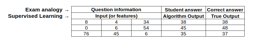
In the above table, you can see how the exam analogy is related to a supervised learning algorithm. Basically, in supervised learning the student is replaced for an algorithm that is trying to predict the correct answer for a question. Additionally, the same way a student learns by answering more questions, a supervised algorithm also learns with more questions. However, in order for it to learn, it is necessary to have a correct answer for each question, so the algorithm can distinguish between a wrong answer and a correct one.
In summary, supervised learning algorithms are capable of predicting an outcome based on some input features. These algorithms have a training process, where they learn what to predict, based on a series of examples with a correct output.
The training process varies depending on the algorithm, nevertheless all of them use a metric to measure how well it is performing against the training examples. This metric can vary a lot depending on the type of model and the objective of the algorithm. For classification models, it is common to use the cross entropy metric, and for regression models, it is common to use the root mean square error (RMSE).
Finally, when working with supervised learning problems, it is common to divide your data in three different sets, when performing a training process. For our example where we can to teach our algorithm to recognize a P300 from other brain waves, you might provide a set of data points corresponding to the P300 brain waves and a set of other brain waves. Then you will divide the data into the training set (used to be fed into the model for training); a validation set (used to evaluate the performance of the model and tune it based on that); and a test set (used for evaluating the final performance of the model). The three separate databases allow us to reduce the bias on our model, so it works well when predicting examples it has never seen before.
Now that we understand a bit more about supervised learning, we can apply this knowledge to train the network that we just created in the previous section.
(Step 3) Create Sample Data
Before we jump into creating a network and training it with the MNE dataset, it is good practice to first test that the network is working correctly with simple, easily classifiable data. The code in this block creates a sample dataset with the same dimensions as the actual data set.
## Create sample data using the parameters
sample_positives = [None, None] # Element [0] is the sample, Element [1] is the class
sample_positives[0] = torch.rand(int(eeg_sample_count / 2), eeg_sample_length) * 0.50 + 0.25
sample_positives[1] = torch.ones([int(eeg_sample_count / 2), 1], dtype=torch.float32)

sample_negatives = [None, None] # Element [0] is the sample, Element [1] is the class
sample_negatives_low = torch.rand(int(eeg_sample_count / 4), eeg_sample_length) * 0.25
sample_negatives_high = torch.rand(int(eeg_sample_count / 4), eeg_sample_length) * 0.25 + 0.75
sample_negatives[0] = torch.cat([sample_negatives_low, sample_negatives_high], dim = 0)
sample_negatives[1] = torch.zeros([int(eeg_sample_count / 2), 1], dtype=torch.float32)

samples = [None, None] # Combine the two
samples[0] = torch.cat([sample_positives[0], sample_negatives[0]], dim = 0)
samples[1] = torch.cat([sample_positives[1], sample_negatives[1]], dim = 0)

## Create test data that isn't trained on
test_positives = torch.rand(10, eeg_sample_length) * 0.50 + 0.25 # Test 10 good samples
test_negatives_low = torch.rand(5, eeg_sample_length) * 0.25 # Test 5 bad low samples
test_negatives_high = torch.rand(5, eeg_sample_length) * 0.25 + 0.75 # Test 5 bad high samples
test_negatives = torch.cat([test_negatives_low, test_negatives_high], dim = 0)

print("We have created a sample dataset with " + str(samples[0].shape[0]) + " samples")
print("Half of those are positive samples with a score of 100%")
print("Half of those are negative samples with a score of 0%")
print("We have also created two sets of 10 test samples to check the validity of the network")
(Step 4) Understand the Sample Data
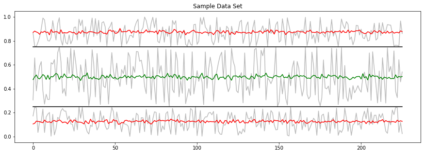
Below is a graph displaying a representation of this dataset. The average of the “good” class 1 samples is represented by the green line. You can see that it is characterized for having values around 0.5 and a larger amplitude than the “bad” class. Two averages of the “bad” class 0 samples are at the top and bottom edges represented by the red lines. We created two “bad” classes, both of them with a smaller amplitude than the “good” classes and centered either around 0.25 or 0.75. An example for each of these classes is plotted in light gray.
We will now design our network around this sample data. If the network classifies this data correctly, it will be more likely to classify the actual, and more complicated, dataset correctly.
rcParams['figure.figsize'] = 15, 5

plt.title("Sample Data Set")
plt.legend()
plt.plot(list(range(0, eeg_sample_length)), sample_positives[0][0], color = "#bbbbbb", label = "One Sample")
plt.plot(list(range(0, eeg_sample_length)), sample_positives[0].mean(dim = 0), color = "g", label = "Mean Positive")
plt.plot(list(range(0, eeg_sample_length)), sample_negatives_high[0], color = "#bbbbbb")
plt.plot(list(range(0, eeg_sample_length)), sample_negatives_high.mean(dim = 0), color = "r", label = "Mean Negative")
plt.plot(list(range(0, eeg_sample_length)), sample_negatives_low[0], color = "#bbbbbb")
plt.plot(list(range(0, eeg_sample_length)), sample_negatives_low.mean(dim = 0), color = "r")
plt.plot(list(range(0, eeg_sample_length)), [0.75] * eeg_sample_length, color = "k")
plt.plot(list(range(0, eeg_sample_length)), [0.25] * eeg_sample_length, color = "k")
plt.show()
(Step 6) Verify the Network Works
Okay, so we’ve trained our network on the sample data and now what’s next? Let’s classify the remaining sample test data to see if the training actually worked.
Below we classify data that the network did not train on to see if it can extrapolate from the training set it did learn from.
# Classify our positive test dataset
predicted_positives = tutorial_model(test_positives).data.tolist()

# Print the results
for index, value in enumerate(predicted_positives):
  print("Positive Test {1} Value scored: {0:.2f}%".format(value[0] * 100, index + 1))

print()

#Classify the negative test dataset
predicted_negatives = tutorial_model(test_negatives).data.tolist()

# Print the results
for index, value in enumerate(predicted_negatives):
  print("Negative Test {1} Value scored: {0:.2f}%".format(value[0] * 100, index + 1))

print()

print("Below is a scatter plot of some of the samples")
print("Notice the distinct areas of red and green dots. If the input of this \n" +
"network was a simple x and y coordinate, the square band in the center would \n" +
"represent the \"solution space\" of our network. However, an actual EEG signal \n" +
"sample is an array of several points and can cross the boundary at any time.")
print("Plotted is one positive sample in green and two negative samples in red")

rcParams['figure.figsize'] = 10, 5
plt.scatter(list(range(0, eeg_sample_length)), test_positives[3], color = "#00aa00")
plt.plot(list(range(0, eeg_sample_length)), test_positives[3], color = "#bbbbbb")
plt.scatter(list(range(0, eeg_sample_length)), test_negatives[0], color = "#aa0000")
plt.plot(list(range(0, eeg_sample_length)), test_negatives[0], color = "#bbbbbb")
plt.scatter(list(range(0, eeg_sample_length)), test_negatives[9], color = "#aa0000")
plt.plot(list(range(0, eeg_sample_length)), test_negatives[9], color = "#bbbbbb")
plt.ylim([0 , 1])
plt.show()
Below is a scatter plot of some of the samples.
Notice the distinct areas of red and green dots. If the input of this network was a simple x and y coordinate, the square band in the center would represent the “solution space” of our network. However, an actual EEG signal sample is an array of several points and can cross the boundary at any time. Plotted is one positive sample in green and two negative samples in red.
It appears that our network is correctly classifying a simple set of fake EEG data is now and ready to be tested out with actual samples. We’re almost ready to solve our P300 problem.
It is left to the reader to perform more experimentation with the sample data by adding overlap between good and bad datasets for example.
(Step 7) Retrieve Data from the MNE EEG Dataset
The MNE library is a resource that specializes in brain signal processing, and provides access to sample databases. We will use one of these P300 databases to train our network.
data_path = mne.datasets.sample.data_path()
data_path
In order to obtain this database using Python, we need to set the path to the specific dataset we are going to use. In this case it is the sample audiovisual database, where the brainwaves have been filtered from 0 to 40 Hz.
The data we obtain is raw. This means that it is simply a collection of streamed brain signal samples from many EEG channels, as opposed to signals sliced or focused to an event of interest.
raw_fname = data_path + '/MEG/sample/sample_audvis_filt-0-40_raw.fif'
event_fname = data_path + '/MEG/sample/sample_audvis_filt-0-40_raw-eve.fif'

# Obtain a reference to the database and preload into RAM
raw_data = mne.io.read_raw_fif(raw_fname, preload=True)

# EEGs work by detecting the voltage between two points. The second reference
# point is set to be the average of all voltages using the following function.
# It is also possible to set the reference voltage to a different number.
raw_data.set_eeg_reference()
Here we load the database and save it in a variable called raw_data. The pick function allows us to choose the sources of interest. For this tutorial we are picking the data from the EEG electrodes. EOG is also included as those are captured using the same electrodes.
This dataset also includes the data from MEG (magnetoencephalography). However, MEG is still very far from being an accessible technology, due to the device being the size of a room. It also requires superconductors to function, similar to fMRI.
# Define what data we want from the dataset
raw_data = raw_data.pick(picks=["eeg","eog"])
picks_eeg_only = mne.pick_types(raw_data.info,
                                eeg=True,
                                eog=True,
                                meg=False,
                                exclude='bads')
The raw EEG file comes with events that allow us to know when something happened during the EEG recording. For example, events with id 5 correspond to when participants were presented with smiley faces, while events 1 through 4 corresponds to trials were participants were presented with a checkerboard either on the left side or the right side of the screen and with a tone presented to either the left ear or the right ear. We know that the trials were participants were presented with a smiley (events with id 5) will elicit a P300. So we will start by slicing (or epoching) the data 0.5 seconds before the image was presented (to have a baseline) and 1 second after the image was presented. We can change this to values closer to 0.3 seconds, which would crop exactly to where the P300 is.
events = mne.read_events(event_fname)
event_id = 5
tmin = -0.5
tmax = 1
epochs = mne.Epochs(raw_data, events, event_id, tmin, tmax, proj=True,
                    picks=picks_eeg_only, baseline=(None, 0), preload=True,
                    reject=dict(eeg=100e-6, eog=150e-6), verbose = False)
print(epochs)
Unfortunately, this dataset only has 12 P300 event examples. Normally, a practical application should have at least 100 examples, but we’ll try anyway.
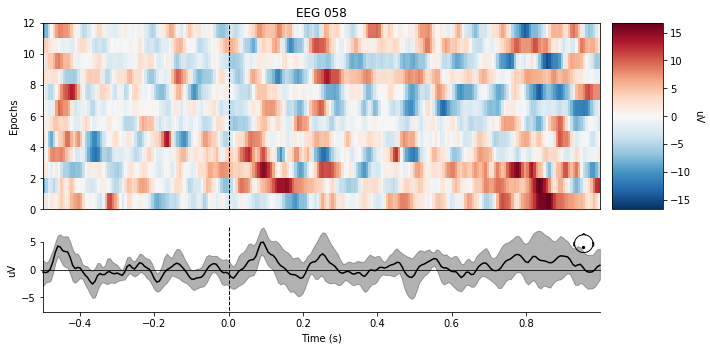
Specifically, we want a single EEG channel that has the highest indication of a P300 component to train our network with. It is possible to use more than one channel, but for simplicity we will use just one in this tutorial. The sensor plot below shows the name of the EEG channel we’re using.
# This is the channel used to monitor the P300 response
channel = "EEG 058"

# Display a graph of the sensor position we're using
sensor_position_figure = epochs.plot_sensors(show_names=[channel])

Below is a heat graph representing the 12 P300 events found within the dataset. If you look closely around the 0.3sec -> 0.4sec mark, you can see there is a noticeable deflection in the signal. That is the P300 component, and the difficulty of detecting it is immediately clear, even with the line graph below the heat graph being the average of the 12 samples.
epochs.plot_image(picks=channel)

Now that we have our P300 component data, we need counter examples to contrast that data with. We’ll gather all of the other miscellaneous events contained within that dataset as well.
event_id=[1,2,3,4]
epochsNoP300 = mne.Epochs(raw_data, events, event_id, tmin, tmax, proj=True,
                    picks=picks_eeg_only, baseline=(None, 0), preload=True,
                    reject=dict(eeg=100e-6, eog=150e-6), verbose = False)
print(epochsNoP300)
There are significantly more Non-P300 events in this dataset, so we will only be using a subset to keep a necessary balance between class data. The most important thing to notice about the plot below is that there is no significant deflection around the 0.3sec -> 0.4sec time interval for the average of the data.
There are significantly more Non-P300 events in this dataset, so we will only be using a subset to keep a necessary balance between class data. The most important thing to notice about the plot below is that there is no significant deflection around the 0.3sec -> 0.4sec time interval for the average of the data.
Here is one more useful all-in-one graph to visualize what these samples look like. Note that the image described in the sample problem earlier in the tutorial is shown at time = 0sec. The blue line corresponds to when the subject was shown a smiley face, and the orange line corresponds to when the subject was shown a checkerboard.
mne.viz.plot_compare_evokeds({'P300': epochs.average(picks=channel), 'Other': epochsNoP300[0:12].average(picks=channel)})

We’ve got a few more steps to take to fully transform our dataset data into something easily digestible by the neural network. We need to:
- Scale the data while being mindful of possible outliers. If we just scale the data using the minimum and the maximum values of our dataset, we run the risk that our data gets defined by outliers and the regular values get squeezed in the center. To avoid this, we can use some statistical values (such as anything a few standard deviations from the mean) to scale our data.
- Create a label variable, where the P300 samples are labeled as 1 and the Non-P300 samples are labeled as 0.
- Combine the data into a single data structure.
- Perform various data type conversions.
The code block below does all of this.
eeg_data_scaler = RobustScaler()

# We have 12 p300 samples
p300s = np.squeeze(epochs.get_data(picks=channel))

# We have 208 non-p300 samples
others = np.squeeze(epochsNoP300.get_data(picks=channel))

# Scale the p300 data using the RobustScaler
p300s = p300s.transpose()
p300s = eeg_data_scaler.fit_transform(p300s)
p300s = p300s.transpose()

# Scale the non-p300 data using the RobustScaler
others = others.transpose()
others = eeg_data_scaler.fit_transform(others)
others = others.transpose()

## Prepare the train and test tensors
# Specify Positive P300 train and test samples
p300s_train = p300s[0:9]
p300s_test = p300s[9:12]
p300s_test = torch.tensor(p300s_test).float()

# Specify Negative P300 train and test samples
others_train = others[30:39]
others_test = others[39:42]
others_test = torch.tensor(others_test).float()

# Combine everything into their final structures
training_data = torch.tensor(np.concatenate((p300s_train, others_train), axis = 0)).float()
positive_testing_data = torch.tensor(p300s_test).float()
negative_testing_data = torch.tensor(others_test).float()

# Print the size of each of our data structures
print("training data count: " + str(training_data.shape[0]))
print("positive testing data count: " + str(positive_testing_data.shape[0]))
print("negative testing data count: " + str(negative_testing_data.shape[0]))

# Generate training labels
labels = torch.tensor(np.zeros((training_data.shape[0],1))).float()
labels[0:10] = 1.0
print("training labels count: " + str(labels.shape[0]))
(Step 8) Classify the Dataset with the Neural Network
Using the network definition created in Step 5, we’ll train on our real EEG data this time, beginning from defaulted weights, prior to any training with the sample data we created.
# Make sure we're starting from untrained every time
tutorial_model = torch.load("/home/tutorial_model_default_state")
## Define a learning function, needs to be reinitialized every load
optimizer = torch.optim.Adam(tutorial_model.parameters(), lr = learning_rate)
## Use our training procedure with the sample data
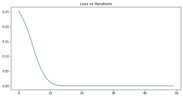
print("Below is the loss graph for dataset training session")
train_network(training_data, labels, iterations = 50)
Alright, the moment of truth! Let’s classify our test data sets.
# Classify our positive test dataset and print the results
classification_1 = tutorial_model(positive_testing_data)
for index, value in enumerate(classification_1.data.tolist()):
  print("P300 Positive Classification {1}: {0:.2f}%".format(value[0] * 100, index + 1))

print()

# Classify our negative test dataset and print the results
classification_2 = tutorial_model(negative_testing_data)
for index, value in enumerate(classification_2.data.tolist()):
  print("P300 Negative Classification {1}: {0:.2f}%".format(value[0] * 100, index + 1))
P300 Positive Classification 1: 100.00%
P300 Positive Classification 2: 99.94%
P300 Positive Classification 3: 100.00%

P300 Negative Classification 1: 99.92%
P300 Negative Classification 2: 0.04%
P300 Negative Classification 3: 0.00%
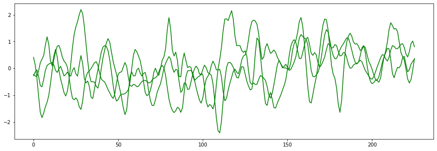
Oh no, while the P300 Positive test samples did very well, one of the P300 Negative samples were misclassified! This is in part a consequence of not having enough data to train on. The network was unable to discern the difference between one of the Negative samples and the rest of the Positive samples. Let’s take a look at what these samples look like next to each other.
rcParams['figure.figsize'] = 15, 5

plt.plot(list(range(0, eeg_sample_length)), positive_testing_data[0], color = "g")
plt.plot(list(range(0, eeg_sample_length)), positive_testing_data[1], color = "g")
plt.plot(list(range(0, eeg_sample_length)), positive_testing_data[2], color = "g")
plt.show()
plt.plot(list(range(0, eeg_sample_length)), negative_testing_data[0], color = "black")
plt.plot(list(range(0, eeg_sample_length)), negative_testing_data[1], color = "r")
plt.plot(list(range(0, eeg_sample_length)), negative_testing_data[2], color = "r")
plt.show()
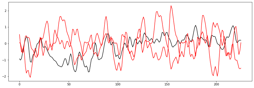
So what happened here? The black line on the second graph is our offender. Visually, it looks similar enough to the Positive samples that it could easily be mistaken for one. Our network would require significantly more examples before it could distinguish samples like this.
Generally, it’s recommended to have at least 100 samples to train on for each class. In this case we only had 9! Not enough for a true application, but enough for a proof of concept. With more samples, the network can develop a more complex and robust solution to classification.
Finishing Remarks
Our network was able to gain some knowledge from the test data provided through the MNE database. Using that knowledge, it was able to predict P300s from brain waves that it had never seen before, and solves our initial problem of detecting surprise in subjects.
Unfortunately, the small amount of data (9 brain waves for each class) to was available to us means that the solution it landed on was not very robust to new unique features. Here is a summary of all the other “Non-P300” data that we didn’t use from the database and the network’s classification of it:
Average Negative Score: 37.79%
Proportion of Non-P300s Classified Correctly: 61.73%
The network performs better than random chance (50%), however there seems to be some room for improvement. This is the result of the network not being complex enough to learn the intricacies of the data, and also not receiving enough examples of what P300s look like. Averaged out, the graphs are easily discernible by the average reader, but individual trials are significantly more ambiguous.
There are a few techniques available to us if we want to improve the network’s performance. These exercises are left to the reader:
- Increase the complexity of the network. This can include more layers, more neurons, more inputs, or altered hyperparameters (For example: modifying learning rate, testing different activation functions, or adding convolutional layers)
- Warning: A consequence in increased complexity in a network is that the network might require significantly more data to train. Also, increasing the learning rate may harbor undesired results.
- Increase the amount of data we train on. There are plenty of free data sets available online which provide a number of different types of data. MNE has a decent number available. Here are a few to try:
- Experiment with different network structures. This technique is by far the most difficult, but since neural networks are just a graph, they can be drawn in any way you’d like! Try out a network that separates the data into two sides. Or a network that has recurrent connections (a loop where two layers feed into each other’s inputs) if you are brave enough. (Warning: it might never return from a training iteration).
So there you have it! We solved our EEG classification problem using a neural network trained on real test data straight from the brain. Thanks for coming along with us on this journey. Now that we have completed our simple example, there are a few more topics that might be interesting to those who would like a little more in depth knowledge on machine learning.
Next steps
Cleaned data:
https://archive.ics.uci.edu/ml/datasets/eeg+database
Advanced topics
Unsupervised learning
Unsupervised Learning methodologies are different from the Supervised Learning methodologies since they do not need any labelled data. Labels are vital for Supervised Learning, but there are situations in which generating or obtaining labelled data could be a problem. While doing academic research or implementing commercial software, you might encounter the following problems when dealing with a dataset:
- No time (or no one) to label your data: EEG data processing requires lots of data. The neurologist labels the EEG data. Sometimes the neurologist is not present in the team or they need too much time to go through all the recordings.
- Not enough data to label: Sometimes there is not enough data for the training set, the validation set and the test set. While developing commercial software, the client is generic and there could be little data available. It’s like buying shoes! You can get the pret-a-porter nice shoes or handmade Italian leather. Pret-a-porter shoes are comfortable and fit everyone. Handmade Italian leather shoes are more expensive and fit only one person, but they fit like a glove. Supervised Learning methods are the latter kind. To remove all the artifacts from the recordings you need to label all the specific person’s artifacts, which takes time and effort. Consumer methods work for everyone’s brain signals, but they don’t fit yours as well as the custom made ones.
Unsupervised learning cuts out calibration, because they do not need labelled data. This reduces the time before online application. It also avoids problems due to wrong labelled data or to miscommunication between training instructor and user during the experiment.
Unsupervised Learning methods are not only an alternative to Supervised methods. They are also a way to get information on a dataset in their own rights.
Unsupervised Learning methods help with signal encoding/decoding and artifacts removal.
The artifacts removal block in the pre-processing rejects the artifacts in the EEG. The most common artifacts are blinking, chewing, frowning and smiling. The EEG channels record the artifacts together with the actual signal and it is a priority to remove as much noise as we can before processing. See the pre-processing lesson for more details.
ICA
The EEG signal has an extremely low SNR, is a non stationary signal and changes from person to person. It has no Gaussian distribution. For this reason Independent Component Analysis is applied: ICA calculates the directions of the subspace by maximizing their non-Gaussianity and separates independent sources, which have been recorded linearly mixed. We can only apply ICA to sources combined linearly. ICA tends to concentrate artifacts, thus it is a good method for artifacts removal. Applying ICA multiple times may improve the quality of the decomposition. In the R function there is the option to have the ica algorithm passed multiple times.
In Independent Component Analysis, the directions have to be statistically independent. Let’s take into consideration the following latent model:
**x** = A**s**
where x is the initial n-dimensional dataset, where n in the number of EEG channels recording the signal. s is composed by l (with l < n ) mutually statistically independent latent variables, which are projected on l independent directions. In this case the signals from all the channels together form the dataset.
The input matrix x represents the collection of the signals from all the channels: voltage difference between channels or between a channel and the reference (usually the electrode on the ear).
ICA also works a priori and has no hypothesis regarding the order of the EEG signals. So you can swap the order of the channels around and the change doesn’t reflect on the processing. So when you input the matrix of the EEG channels you don’t need to worry about the cables order.
The output matrix s contains the independent components, the mutually statistically independent latent variables. Therefore you can isolate domains of cortical synchrony.
A is called mixing matrix.
We aim to find the vector of lower dimension variables and the values of these variables in the new subspace. This subspace’s dimension will be lower than the one we previously had.
ICA example by the MNE library:
Details on ICA Methods
Infomax is a method based on maximizing the joint entropy of a nonlinear function of the estimated source signals. See Bell and Sejnowski (1995) and Helwig (in prep) for specifics of algorithms.
FastICA is a method based on maximizing the negentropy of the estimated source signals. Negentropy is calculated based on the expectation of the contrast function. See Hyvarinen (1999) for specifics of fixed-point algorithm.
JADE calculates the subspace by diagonalizing the cumulant array of the source signals. See Cardoso and Souloumiac (1993,1996) and Helwig and Hong (2013) for specifics of the JADE algorithm.
Example:
In the following example, 3 signals will be artificially created and mixed. Then, we will process the signals with ICA and see how it works.
Python
There are many useful libraries in this case, depending on the level of coding you want to apply and implement. We are going to review MNE, which is specific for EEG.
mne.processing.ICA class implements ICA with four different methods: fastica, picard, infomax, and the extended-infomax algorithm. Bad data segments can be rejected by reject parameter mne.preprocessing.ICA.fit.
#Import required libraries for generating the sample signals
import numpy as np
import matplotlib.pyplot as plt
from scipy import signal

#Creating sample signals

np.random.seed(101)
size = 5000
time = np.linspace(0, 8, size)

signal1 = np.sin(2 * time)
signal2 = signal.sawtooth(2 * np.pi * time)
signal3 = np.sign(np.sin(3 * time))

final_signal = np.vstack((signal1, signal2, signal3)).T
final_signal += 0.2 * np.random.normal(size=final_signal.shape)  # Add noise

# Mix signals data
A = np.array([[1, 1, 1], [0.5, 2, 1.0], [1.5, 1.0, 2.0]])  # Mixing matrix
mixed_signal = np.dot(final_signal, A.T)  # Generate observations


#Importing libraries to process signals
from sklearn.decomposition import FastICA, PCA

#PCA processing
pca = PCA(n_components = 3)
pca_signal = pca.fit_transform(mixed_signal)

#ICA processing
ica = FastICA(n_components=3)
ica_signal = ica.fit_transform(mixed_signal)


#Ploting data

fig, axs = plt.subplots(4,1, figsize=(10, 3*4))

#1st: Raw signal

ax = axs[0]
ax.set_title('Real signals')
ax.plot(np.arange(len(final_signal)), final_signal[:,0])
ax.plot(np.arange(len(final_signal)), final_signal[:,1])
ax.plot(np.arange(len(final_signal)), final_signal[:,2])

#2nd: Mixed signal

ax = axs[1]
ax.set_title('Mixed signals')
ax.plot(np.arange(len(mixed_signal)), mixed_signal[:,0])
ax.plot(np.arange(len(mixed_signal)), mixed_signal[:,1])
ax.plot(np.arange(len(mixed_signal)), mixed_signal[:,2])

#3rd: PCA signal

ax = axs[2]
ax.set_title('PCA result')
ax.plot(np.arange(len(pca_signal)), pca_signal[:,0])
ax.plot(np.arange(len(pca_signal)), pca_signal[:,1])
ax.plot(np.arange(len(pca_signal)), pca_signal[:,2])

#4th: ICA signal

ax = axs[3]
ax.set_title('ICA results')
ax.plot(np.arange(len(ica_signal)), ica_signal[:,0])
ax.plot(np.arange(len(ica_signal)), ica_signal[:,1])
ax.plot(np.arange(len(ica_signal)), ica_signal[:,2])

plt.tight_layout()
plt.show()
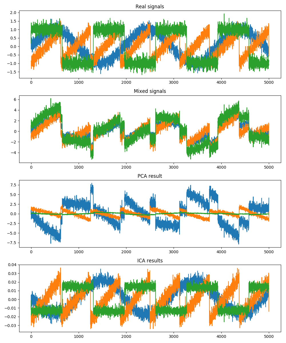
As it is possible to observe from the image above, when having the mixed signal, it is very difficult to distinguish between each of the 3 components. When the PCA process is applied, it is possible to clearly discern the individual components. Nevertheless, they do not follow the same pattern as the real data. Finally, we can see why ICA is most commonly used on this type of problems, as each one of the components obtained has the same kind of signal profile as the initial data.
# init ICA. Feed dataset, method and random_state

ica =<span style="text-decoration:underline;"> </span>ICA(n_components=n_components, method=method, random_state=random_state)

# define what kind of components you want to reject

reject = dict(mag=5e-12, grad=4000e-13) \
ica.fit(raw, picks=picks_meg, decim=decim, reject=reject) \
ica.plot_components()

# i.e., to plot component 0:
ica.plot_properties(raw, picks=0)
R
eegkit package implements ICA methods in R. Methods available are “imax”, “fast”, and “jade”
ica =<span style="text-decoration:underline;"> </span>eegica(n_components = n_components(rows = channels, cols = time points), nc, center = TRUE, maxit = 100, tol = 1e-6, Rmat = diag(nc), type = c(“time”, “space”), method = c(“imax”, “fast”, “jade”)
nc is the number of components to extract. If center is TRUE then the functions mean-centers the columns before decomposition. maxit is the maximal number of algorithm iteration allowed. tol is the convergence tolerance. Rmat Initial estimate of the nc-by-nc orthogonal rotation matrix.
MATLAB
The all inclusive EEG toolkit in MATLAB is EEGLAB. The user-friendly method to apply ICA is to call the function pop_runica and select variables and dataset directly from the pop up window. At this point the only options in EEGLAB are runica - which uses infomax - and jade. To use the function fastica, you need to install the fastica toolbox. Let’s also mention the faster version of runica, called binica. Both give stable decomposition while processing hundreds of channels.
Details on ICA Methods
Infomax is a method based on maximizing the joint entropy of a nonlinear function of the estimated source signals. See Bell and Sejnowski (1995) and Helwig (in prep) for specifics of algorithms.
FastICA is a method based on maximizing the negentropy of the estimated source signals. Negentropy is calculated based on the expectation of the contrast function. See Hyvarinen (1999) for specifics of fixed-point algorithm.
JADE calculates the subspace by diagonalizing the cumulant array of the source signals. See Cardoso and Souloumiac (1993,1996) and Helwig and Hong (2013) for specifics of the JADE algorithm.
Clustering Component Analysis
Clustering methods can further develop the independent component analysis. When confronted with a pool of subjects, multiple sessions or different protocols, it might be useful to do a cross analysis. In case of software development, clustering the independent component analysis results could be useful for checking the results in real time and finding out outliers.
Clustering is a method in Unsupervised Learning which allows you to group together elements with some commonalities. Usually we tend to cluster elements that have similar values for a specific feature. To do so the best technique is k-mean. It is demonstrated that this is the most efficient method to cluster elements.
Python / R
There are several steps in the independent component clustering process:
Identify a set of epoched EEG datasets for performing clustering.
[Optional] Specify the subject code and group, task condition, and session for each dataset.
Identify components to cluster from each dataset.
Specify and compute measures to use to cluster (pre-clustering).
Perform clustering based on these measures.
View the scalp maps, dipole models, and activity measures of the clusters.
[Optional] Perform signal processing and statistical estimation on component clusters.
MATLAB
EEGLAB v5.0b has a new structure called STUDY. It allows to store different subjects, sessions and so on. It also allows to compare features between subjects, sessions and protocols. The function that allows clustering component analysis is ICACLUST.
Online vs Offline applications
Depending on the industry and the task, you may find yourself processing either real-time or offline.
Usually experimental procedures used during research oriented experiments work on data gathered from subjects screened. Such data is previously recorded and then used later on. So research and most of accademia related software processes data offline.
On the other hand, when designing and developing software, real time could be one of the requirements of the algorithm. In this scenario, the software needs to be tested before reaching the consumer. Testing protocols require a dataset already labelled to check the results and compare them to the software output. Therefore in both examples there is a dataset available.
The presence of the dataset doesn’t automatically mean “Supervised Learning”. Software using “Unsupervised Learning” methodologies might be tested on previously recorded dataset before being released. It could be a very short dataset! Or not yet labelled. But the combination of offline - real time allows other strategies to be actualized.
Combining classifiers
Bagging
The idea of bagging comes from a classic example that occurs frequently in the real world.
Given some phenomenon that produces data, say time delay between stimulus and ERP response, I might collect some data from my observations and you might collect some data from your observations. We then fit our models via regression to predict the time delay based on various factors (age, weight, etc). However, it may turn out that the data we collect is localized due to some unforeseen factors (perhaps you used right handed subjects and I used left handed ones). In this instance, it is highly likely for any models that we build to lean towards the low bias, high variance, overfitted side of the bias-variance trade off. In other words, we overfit to the data we have collected and thus our models do not generalize well to the general population.
Having encountered this problem, one solution might be to average our model parameters such that we have a new model that incorporates both of our data sets. This is the idea of bagging: to overfit many low bias, high variance models, then average to reduce variance.
In practice, bagging is often used in conjunction with nonparametric techniques that often have high variance, canonical decision trees (i.e. random forest) but also k-nn, etc. Given some dataset, we take many samples via bootstrapping, and model each sample in parallel, overfitting every sample. We then average all the models together, and in theory, this leads to the same bias (low by default) while reducing the variance roughly by a factor of 1/M (M= number of samples). This rarely happens in practice - see the Cornell lecture regarding stable learners for more details.
Boosting
Another common scenario may play out as follows.
Knowing about bagging, I split my dataset into some subsets. I fit some initial submodels and average, then predict some initial results. However, the performance may still be mediocre. This could be a case where the model leans towards the high bias, low variance side of the bias-variance trade off. Our initial submodels are too simple and do not capture the characteristics of the data; the models are under fitted.
One thing I might do to improve performance is to study some model fit indicators, for example, residuals, to investigate how to better tune the submodels. I then make adjustments to my original submodels based on the results of my investigations. To really put my submodels to the test, I select data which I know my previous model struggled with - the ‘hard’ data points - and use these as new subsets to train my new submodels on. I aggregate (weighted average of each submodel) and produce a new model which fits better than the original. I repeat this process as necessary, updating my weights to preserve the good base models. This is the idea of boosting: sequentially fitting better and better sets of base models based on the residuals of the previous trials.
In practice, boosting has proven effective in reducing bias and improving predictive power. It was a very popular option in contests due to its ease of implementation and its flexibility, to the point where there was a period of time when many competitions were only won by boosting algorithms. However, since boosting requires the sequential fitting of models as well needing to choose the ‘hard’ data points, it is computationally expensive. XGBoost is a popular gradient boosting tree package in Python.
Stacking
Until now, we have supposed that each of the base models described in the above sections were uniform (i.e. if we are bagging, the models we average are all decision trees). However, this need not be the case. Stacking refers to the technique whereby many different models are combined. In this case, a meta layer must be added to introduce a ‘reward’ mechanism for good models and a ‘punishment’ for poor models. This meta layer contains weights for each of the base models. Each base model predicts a value for the final outcome and then the values are multiplied by weights, then combined (usually via a logistic function) into a final result. The weights as well as the base models parameters are then adjusted based on feedback (e.g. stochastic gradient descent) and the theory is that eventually, the poor models are weeded out and only the powerful ones remain. Stacking can be thought of as boosting different models, but a good approach to tune the meta layer as well as propagate the errors back to the base models makes stacking much more difficult to implement in practice.
Recommended Resources
Libraries for machine learning for python:
Library to analyze EEG data
https://mne.tools/stable/index.html
Sample EEG data to play with:
Library to process EEG data with Deep Neural Networks
https://github.com/kylemath/DeepEEG
Amazing BCI applications
    [https://www.biorxiv.org/content/biorxiv/early/2017/12/30/240317.full.pdf](https://www.biorxiv.org/content/biorxiv/early/2017/12/30/240317.full.pdf)


    [https://www.nature.com/articles/nn1444](https://www.nature.com/articles/nn1444)
1 Hour Master Class on the challenges for Brain Computer Interfaces
https://www.youtube.com/watch?v=5gOhNV6woT0
For computer scientists: How is analyzing EEG data different from analyzing images?
https://arxiv.org/abs/1901.05498
Explanation of how to use neural networks on BCI applications
Explanation of convolutional neural networks
https://adeshpande3.github.io/A-Beginner%27s-Guide-To-Understanding-Convolutional-Neural-Networks/
Library to benchmark different algorithms: Mother of All BCI Benchmark
http://moabb.neurotechx.com/docs/
Simulation of vital signals to use in different analyzes
https://physiology.kitware.com/
Classes and tutorials on machine learning and cognitive science
https://tomdonoghue.github.io/teaching.html
https://github.com/voytekresearch
Examples using the commercial EEG Headset Muse
https://github.com/NeuroTechX/eeg-notebooks
Machine learning library specialized in neuroimaging, particularly fMRI
Data Structure for fMRI
Tutorial in Google Colab to analyze fMRI data using the library Keras
https://github.com/NeuroTechX/minc_keras
Resources for combining classifiers.